Sweep waveguide width
Compute the effective index of different modes for different waveguide widths
we compute mode properties (neff, aeff …) as a function of the waveguide width
we have to make sure that the simulation region is larger than the waveguide
Simulation of mode hybridisation in 220nm thick fully-etched SOI ridge waveguides.
Results look the same as those found in Daoxin Dai and Ming Zhang, “Mode hybridization and conversion in silicon-on-insulator nanowires with angled sidewalls,” Opt. Express 23, 32452-32464 (2015).
_________________________________

                                clad_thickness
       width
     <---------->
      ___________    _ _ _ _ _ _
     |           |
_____|           |____          |
                                wg_heigth
slab_thickness                     |
_______________________ _ _ _ _ __

sub_thickness
_________________________________
<------------------------------->
             sub_width
[1]:
import numpy as np
import matplotlib.pyplot as plt
import modes as ms
import opticalmaterialspy as mat

#widths = np.arange(0.3, 2.0, 0.02)
widths = np.arange(0.3, 2.0, 0.2)

wgs = [ms.waveguide(width=width) for width in widths]
wgs[0]
[1]:
0.3 x 0.22 um, n_wg = 3.4757, n_clad = [1.444023621703261]

[2]:
s = ms.sweep_waveguide?
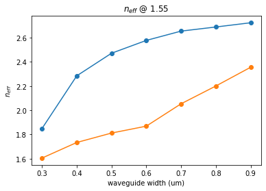
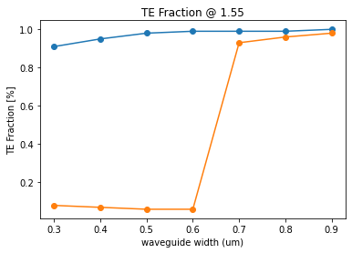
1550 nm strip waveguides
Here are some waveguide simulations for C (1550nm) and O (1310) band, where we sweep the waveguide width and compute the effective modes supported by the waveguide.
TE mode (transverse-electrical) means that the light is mainly polarized in the horizontal direction (the main electric field component is Ex) while TM transverse magnetic field modes have the strongest field component (Ey). We can see why for 1550nm a typical waveguide width is 0.5nm, as they only support one TE mode.
[3]:
ms.mode_solver_full?
[4]:
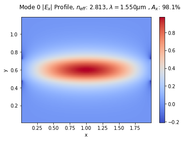
ms.mode_solver_full(width=0.5, plot=True, plot_index=True, fields_to_write=('Ex', 'Ey'))
[4]:
<modes._mode_solver_full_vectorial.ModeSolverFullyVectorial at 0x7f068041d400>


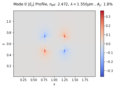
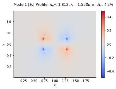

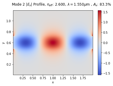
As waveguides become wider they start supporting more than one single mode. For example, a 2um wide waveguide supports 4 different TE modes (TE0: 1 lobe, TE1: 2 lobes, TE2: 3 lobes, TE3:4 lobes)
[5]:
ms.mode_solver_full(width=2.0, plot=True, plot_index=True, n_modes=4, fields_to_write=('Ex'))
[5]:
<modes._mode_solver_full_vectorial.ModeSolverFullyVectorial at 0x7f067fb39d30>


[6]:
s = ms.sweep_waveguide(wgs, widths, legend=['TE0', 'TM0', 'TE1', 'TM1'], overwrite=False)
100%|███████████████████████████████████| 9/9 [00:16<00:00, 1.85s/it]
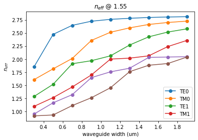


we can create a waveguide compact model that captures the neff variation with width for the fundamental TE mode
[7]:
s.keys()
[7]:
dict_keys(['n_effs', 'mode_types', 'fractions_te', 'fractions_tm'])
[8]:
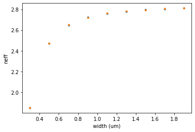
n0 = [n[0] for n in s['n_effs']]
[9]:
plt.plot(widths, n0, '.')
plt.xlabel('width (um)')
plt.ylabel('neff')
[9]:
Text(0, 0.5, 'neff')

[10]:
p  = np.polyfit(widths, n0, 6)
n0f = np.polyval(p, widths)
plt.plot(widths, n0, '.')
plt.plot(widths, n0f, '.')
plt.xlabel('width (um)')
plt.ylabel('neff')
[10]:
Text(0, 0.5, 'neff')
[11]:
p
[11]:
array([ -1.55850963,  11.5812411 , -35.03432244,  55.35340064,
       -48.51250016,  22.76471863,  -1.85178724])
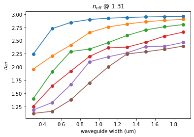
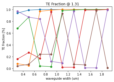
1310 nm strip waveguides
[12]:
wgs1310 = [ms.waveguide(width=width, wavelength=1.31) for width in widths]
[13]:
s = ms.sweep_waveguide(wgs1310, widths)
100%|███████████████████████████████████| 9/9 [00:16<00:00, 1.79s/it]

[14]:
widths = np.arange(0.3, 1.0, 0.1)
overwrite = False
wgs = [ms.waveguide(width=width) for width in widths]
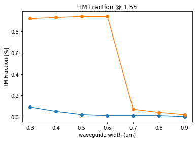
r2 = ms.sweep_waveguide(
wgs, widths, n_modes=2, fraction_mode_list=[1, 2], overwrite=overwrite,
)
100%|███████████████████████████████████| 7/7 [00:05<00:00, 1.34it/s]
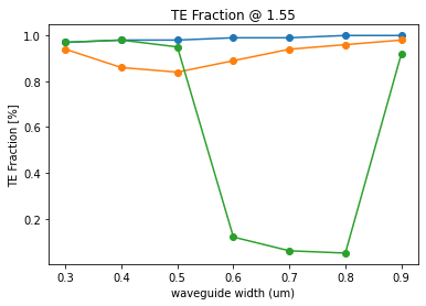
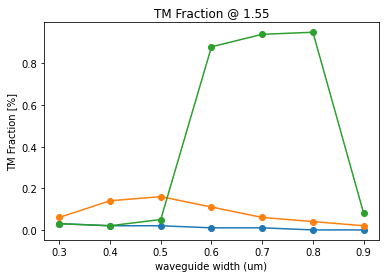
Rib waveguide sweep
For 90nm slab
[15]:
widths = np.arange(0.3, 1.0, 0.1)
overwrite = False
wgs = [ms.waveguide(width=width, slab_thickness=90e-3) for width in widths]
r2 = ms.sweep_waveguide(
    wgs, widths, n_modes=3, fraction_mode_list=[1, 2, 3], overwrite=overwrite,
)
100%|███████████████████████████████████| 7/7 [00:07<00:00, 1.11s/it]